How to Make a Drop-Down List in Excel?

Drop-down lists in Excel are essential for making data entry more efficient and maintaining consistency. They're not only time-saving, but also add interactivity and accuracy to your spreadsheets. Whether you're handling a small project or organizing extensive datasets, drop-down lists can help keep things organized.

What Is a Drop Down List?

An Excel drop-down list is a tool that makes data entry easier. It allows users to select from a set of options instead of typing. When I want users to choose from predefined options, I create a drop-down list. It works by showing a down arrow next to a selected cell, and clicking on it displays all the available choices. It's a great way to prevent users from entering incorrect values. It's part of Excel's data validation features, which control what can be entered in a cell to ensure accuracy and consistency.

Benefits of Using Drop Down Lists

By learning how to make a drop down list in Excel, I have several benefits. For instance, if I need to create a sales report that requires referencing specific product categories for each entry, setting up a drop down list with all the categories ensures that:

• Data Entry Speed: I boost efficiency by avoiding the need to repeatedly type the same information.
• Error Reduction: Typing mistakes are minimized since the options are pre-defined and selectable.
• Consistency: Everyone working on the document selects from the same list, which leads to uniform data across the board.

Couple these benefits with user-friendly interfaces and drop down lists transform a basic spreadsheet into a more powerful and interactive tool. For instance, in project management trackers, I've seen drop down lists perform excellently in preventing any discrepancies that could muddy the analysis of crucial data. Using conditional formatting in tandem with drop down lists elevates the functionality, allowing me to set visual cues for correct or incorrect entries.

The dynamic nature of drop-down lists, especially with dependent lists in Excel 2021, adds sophistication. For example, if you have a document with company branches, cities, and countries, setting up cascading drop-down lists will automatically narrow down the city selection when a country is chosen. This makes data handling easier and more streamlined.

I find drop down lists very useful in Excel for organizing large datasets and improving user interaction. I rely on them regularly when creating forms for data collection or working on complex financial models. They help me manage information more accurately and with less hassle.

Creating a Drop Down List in Excel

Step 1: Open Excel and Select a Cell

When starting the process, I open my Excel worksheet and click on the cell where I want my drop-down list to appear. This prepares that specific cell for the data I’ll input.

Step 2: Go to the Data Tab

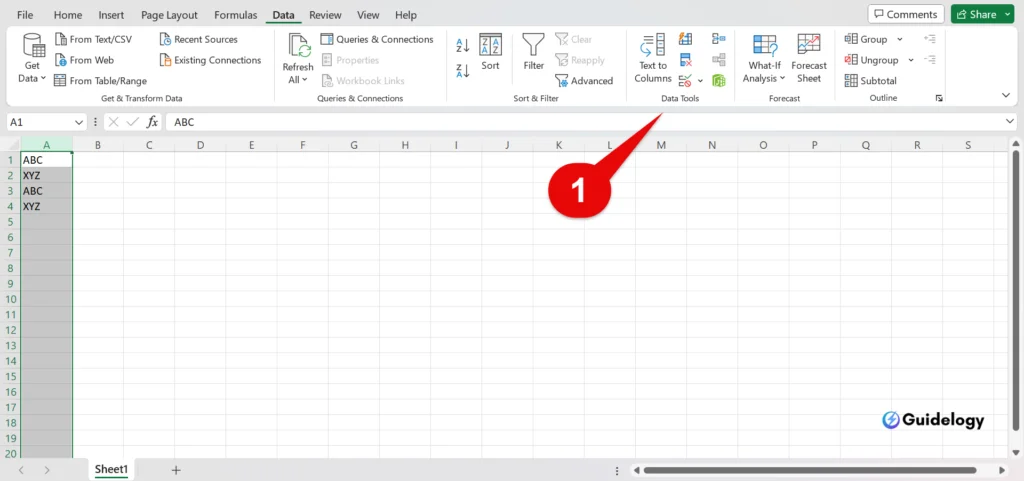
Next, I navigate to the Data tab at the top of the screen. It's crucial because this tab contains the tools I need for creating a drop-down list in Excel.

Step 3: Click on Data Validation

On the Data tab, I click on the Data Validation button in Data Tools. This takes me to the settings that allow me to define what data can enter into my selected cell.

Step 4: Enter the Values for Drop Down List

Now I get to the core part where I enter the values I want in my drop-down list directly into the Source box or select the range that holds the values. I make sure to use commas if I'm typing them out manually to separate each item.

Step 5: Click “OK” to Save

After entering all my values, I click “OK” to finalize the creation of my drop-down list. Now, whenever I or anyone else clicks on that cell, a list of pre-defined options appears for easy selection.

Customizing the Drop Down List

When I jump into how to create a drop down list in Excel, I also make sure to customize my list. This optimizes data entry and enhances the user experience. Below, I'll detail how to limit input, title your list, and tweak its appearance for Excel 2021 and beyond.

Restricting Input to the List

Allowing only certain inputs in a drop down ensures data integrity. Here's how it's done:

• Open the Data Validation dialog box by clicking on Data Validation in the Data Tools group.
• Choose the List option under the Allow field.
• Ensure that the Error Alert tab is configured to disallow entries not on the list by selecting ‘Stop'.

This effectively restricts users to the predefined list, reducing errors and maintaining consistency across dataset entries.

Adding a Title to the Drop Down List

A title gives users context. Here's how to add a title:

• Click on the Input Message tab within the Data Validation dialog box.
• Input a straightforward title in the Title field.
• Add a brief message to guide users.

With a limit of 225 characters for the input message, it's key to be succinct yet informative.

Changing the Appearance of the Drop Down List

To alter the list's style, you'll find the following steps useful:

• From the Data Validation menu, hit the Settings tab.
• Choose Format Cells to change font, color, or add borders to your drop down.

Remember that a visually appealing drop down list not only helps in sustaining user attention but also assists in quick data retrieval.

Through these methods, I can confidently create a drop down list in Excel 2021 that is both functional and well-designed, enhancing the overall usability of my spreadsheets.

Using the Drop Down List in Excel

Selecting an Item from the List

Once I've mastered how to create a drop down list in Excel, selecting an item from it couldn't be easier. Clicking on the cell that contains the list activates a small arrow on the right side of the cell. Simply click on this arrow, and a list of predefined options appears. Choosing an item is as simple as clicking on the desired option.

For instance, if I've created a list containing cities like New York, Boston, and Los Angeles, I just click the drop down arrow next to the cell and select the city I need to input. This method is user-friendly and gives a significant boost to data entry efficiency by minimizing the risk of typographical errors. It ensures data consistency, particularly when I'm working with large datasets where manual entry could lead to discrepancies.

Sorting and Filtering Data with the Drop Down List

The functionality of drop down lists extends beyond mere selection. I can sort or filter data in Excel based on the options within the drop down list, making it an invaluable asset for data analysis. Say I have a spreadsheet filled with sales data for different products. By incorporating a drop down list to categorize products, I can quickly filter the entire worksheet to display only the data relevant to the selected product.

Here's how I sort data using a drop down list:

• After creating a drop down list in Excel 2021, I ensure that my source data is appropriately organized.
• Using Excel's built-in sorting feature, I can rearrange the data alphabetically or numerically based on the items selected from the drop down.

For example, to arrange my sales data by product name, I'll go to the Data tab, click Sort, and select my drop down list as the reference for sorting. This reorganizes my data swiftly, displaying it in a more digestible format. Filtering follows a similar process where I use the filter option to display only rows that match my drop down list selection, aiding in a precise data review.

Do I Need a Formula to Create Drop-Down Lists?

When working with Excel, there is no single approach that works for everyone when it comes to creating a drop-down list. Whether or not you need a formula depends on the specific situation.

Understanding the Basics

For standard drop-down lists where I want users to select from a fixed set of text options, formulas aren't necessary. I find this method perfect for situations where the options don't change, like a list of company departments or days of the week.

The Power of Dynamic Drop-Down Lists

If you need a spreadsheet that can change in size or options over time, it's best to use formulas. Formulas can make your list automatically update as you add or remove items, saving you from having to update it manually.

Real-Life Application

Imagine you want to make a drop-down list in Excel that updates the nutritional information depending on the serving size I choose. By using the Define Name command and the OFFSET function, I can easily achieve this.

First, I create named ranges using the Define Name command. This lets me refer to those ranges within my worksheet. If I change the food amount from 100g to 80g, a formula connected to my drop-down list will automatically adjust the macros.

Creating a Drop-Down List With Images

I have tried making drop-down lists more visually appealing by adding images or icons. It's a bit more complex than using plain text, but by formatting cells creatively and using VBA code, it can be done.

Dynamic Lists and OFFSET Function

For those who prefer a more technical approach, Excel's OFFSET function is a life-saver. This formula is essential when I'm creating a drop-down list that automatically includes new data entries. I prefer this method as it saves time and reduces the potential for errors in my data sets.

To illustrate, here are the steps I take to use the OFFSET function for a dynamic list:

• I define the desired range for my list using the Define Name tool.

Make a Dynamic Dropdown List in Excel 365/2021

Creating a dynamic dropdown list in Excel is a game-changer for managing spreadsheets efficiently. With Excel 365/2021, this task is more user-friendly than ever, ensuring that your dropdown menus are not just static but evolve as your data does.

Excel Tables and Dynamic Lists

Instead of using a simple range, Excel tables offer a spectacular way to manage dynamic drop-down lists. Here's the beauty of it—I don't have to worry about any changes made to the list. It's all taken care of automatically as I add or remove items. For instance, if I'm managing a project inventory, and a new item arrives, I drop it into the Excel table and, like magic, it's reflected in the dropdown list without any additional steps.

Use the UNIQUE Function

Another standout feature in Excel 365/2021 is the UNIQUE function. It's perfect for when I need to exclude duplicates from my dropdown list, ensuring every item is just listed once. If I'm organizing an event and need to list unique venues available, the UNIQUE function is my go-to tool. It saves time and avoids any confusion with repeat entries.

Creating a Linked Dropdown List Across Sheets

Excel's dynamic dropdown capabilities aren't confined to a single sheet. I can easily link dropdown lists across different worksheets, which means I can select an item on one sheet and see related content dynamically update in another. This comes in handy for comprehensive datasets where I need interconnected information accessible at a glance.

Managing Dynamic Dropdowns Across Workbooks

In some cases, the data for my dropdown list might be housed in a different workbook entirely. With Excel 365/2021, I can create a link using the OFFSET formula. Any updates I make in the source workbook are automatically reflected in the dropdown menu of the connected workbook—a real time-saver when dealing with complex datasets that span multiple files.

Quick Tips for Dropdown List Efficiency

• Always name your ranges or tables—you'll thank yourself when you need to review or modify data sources later on.
• Check for the latest updates in Excel 365/2021 to ensure all the dynamic functions are at your disposal.
• Familiarize yourself with formulas like OFFSET and UNIQUE as they're central to creating these living, breathing dropdown lists.

How to Make Drop-Down List From Another Workbook

If you've ever managed data across multiple Excel workbooks, you'll understand the significance of streamlining data entry. It's common to use a drop-down list in a primary workbook that refers to data in a different workbook. The process varies slightly from creating a drop-down list within a single workbook but can be mastered easily.

To start, in the main workbook, select the cell where you want your drop-down list. Go to the Data tab and choose Data Validation. In the dialog box, under the Settings tab next to the Source, you’ll enter the reference to the external list. Let's say the list is named ‘Items' in the source workbook. You will type =Items to link to that named range.

Keep in mind that for the external drop-down list to function correctly, the workbook containing the source data must be open. This is a crucial step to ensure that the data feeding your list is accessible and current.

Dynamic Drop-Down Lists

Creating a static list is straightforward, but imagine you need to update your list by adding new items frequently. That's where dynamic drop-down lists come into play. By using a Named Range with the OFFSET function, any changes made to the data in the source workbook will reflect in your list automatically. Here's how you can set up a dynamic named range:

• Open the workbook with the source list.
• Use the OFFSET formula within Name Manager to define the range dynamically.
• Name the range, and this name will be your source reference for the drop-down in the other workbook.

Any adjustment to the master list in the source workbook dynamically updates the dependent drop-down list. This method ensures that your lists remain up to date without continuously modifying range references manually.

Adding New Items

When you're dealing with a named range, adding new items might require a bit more attention. You need to extend your named range to include these new elements, which you can seamlessly manage through the Name Manager. It's a simple edit but essential for maintaining the integrity of your data-driven lists.

How to Create Drop Down List From Another Sheet

When working with Excel, creating a drop down list from another sheet is a common task that streamlines data management. I'll walk you through the process using a practical example to ensure you can apply these steps to your own work.

Let's assume I'm managing an inventory spreadsheet, and I need staff to select products from a drop down list. The list source is on a sheet named ‘Products', while the selections are made on the ‘Inventory' sheet.

Step 1: Set Up the Source Sheet

First, I need to make sure my product list is up-to-date. I'll go to the ‘Products' sheet and format my list as an Excel Table. Excel tables are ideal for dynamic lists because they automatically expand when new items are added, ensuring nothing is omitted from the drop down list.

Step 2: Name the Range

After creating the table, I'll select the range of cells containing the product names and define a named range. To do this, I simply type the name ‘ProductList' into the Name Box above the spreadsheet and hit Enter. This name will be used to reference the product list from the ‘Inventory' sheet.

Step 3: Create the Drop Down on the Destination Sheet

I'll switch over to the ‘Inventory' sheet where the drop down is needed. In the cell where I want the list to appear:

• I'll navigate to the Data tab, – Click on Data Validation in Data Tools, – And in the Source box, I'll type ‘=ProductList'.

Since the source data is on a different sheet, Excel understands that ‘ProductList' is a named range and automatically retrieves the correct items.

Step 4: Ensure Dynamic Updating

By linking the drop down list to a named range on a table-formatted list, any changes in the ‘Products' sheet automatically reflect in the ‘Inventory' drop down. This is crucial for maintaining accurate records and making sure everyone's on the same page—literally. If I add a new product to the ‘Products' table, it's instantly available in the ‘Inventory' sheet's drop down menu without any additional steps.

How Do I Create a Yes/No Drop-Down in Excel?

When working with data entry tasks, simplicity and efficiency are key. That's where a yes/no drop-down list in Excel becomes indispensable. Let's jump into the process that'll save time and reduce input errors.

Imagine this: I'm managing a feedback form and I need to record responses as either ‘Yes' or ‘No'. Here's how I simplify the process by creating a straightforward drop-down list for quick and easy data input. First, I choose the cells where I want the drop-down list. Instead of typing the responses manually, I click on Data Validation in the Data tab. I simply enter ‘Yes,No' (without any spaces) in the Source field. That's all it takes to set up this type of drop-down. By following these simple steps, I ensure that my feedback form is error-proof and prevents any inconsistent data entries.

Is a Drop-Down List the Same as Data Filtering?

When managing data in Excel, it's common to confuse drop-down lists with data filtering, though they serve different functions. I'll clarify the distinctions to ensure you're equipped with the correct tools for your tasks.

Creating a drop-down list in Excel and setting up data filters might seem similar since both involve making selections from a range of options. But, a drop-down list is essentially a tool that confines input to set values within a cell. It's what I use when I need to standardize entries and avoid errors from manual typing. For instance, if I'm handling an inventory spreadsheet, I can create a drop-down list for product categories to ensure consistency in my records.

On the other hand, data filtering allows me to sift through a dataset and display only the rows that meet certain criteria. Think of it as a way to declutter a packed spreadsheet to showcase only the relevant information. As an example, if I've got a comprehensive sales report, I can apply a filter to display only transactions above a specific value, or from a certain region.

It's important to mention that while filters are excellent for analysis, they don't restrict data entry like drop-down lists do. So when it comes to actual data input and maintaining the integrity of your data sets, that's where learning how to create a drop-down list in Excel becomes critical. As of Excel 2021, creating these lists has become more intuitive, allowing users to efficiently manage data input without extensive expertise in Excel functions.

Besides, while filters can be applied and removed on the fly, affecting the view of the dataset, a drop-down list is a permanent feature of the cell unless explicitly removed. This means that whether I'm sorting or searching through data using filters, the drop-down list remains intact, guiding data entry at every step.

The creation process of a drop-down list in Excel, particularly in the 2021 version, hinges on the Data Validation tool. This feature doesn't intersect with the filtering process, ensuring that both tools can operate independently within the same sheet.

Conclusion

Mastering drop-down lists in Excel can streamline your data entry and ensure consistency across your datasets. Remember, while these lists offer a straightforward way to manage your data, they're just one part of the Excel toolkit designed to enhance your productivity. With practice, you'll find incorporating drop-down lists into your spreadsheets becomes second nature. Don't hesitate to revisit these steps whenever you need a refresher or share this knowledge to empower others in their data management endeavors. Excel's capabilities are vast and with each skill you acquire you're not just improving your spreadsheets—you're boosting your analytical prowess. Keep experimenting and watch your efficiency soar!

Frequently Asked Questions